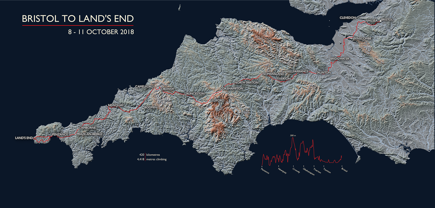
Last autumn I undertook my first cycle tour: from Bristol to Lands End, Cornwall over 4 days. I thought it would be good to remember the ride by making a map of the route for the wall. This became a bit more involved than expected…

Download OS Open Data

I decided to use OS Open Data as the main source for the map. This is a fantastic free resource offered by the Ordnance Survey. I used their OS Terrain 50 gridded digital terrain model, OS Open Rivers and OS Open Names datasets. These data are fairly simple to download following a quick registration process.

Prepare OS Open Data for use

Once downloaded the data all need to be unzipped. Some OS Open Data are divided into tiles according to the OS National Grid System which covers the UK using twenty-five 100 x 100 km tiles. Several tiles are therefore needed to cover the West Country and the data need unzipping before use (sometime unzipping zip files within zip files). With Unix, for the OS Terrain 50 product this can be done in a way similar to this:

cd /path/to/terrain50
unzip main_terrain50.zip
for f in */*zip; do unzip $f; done

To stitch the OS Terrain 50 data for the west country I used gdal_merge.py, supplying it with all the *.asc files and setting the -ul_lr option to an extent appropriate to the west country. This produced a mosaiced DTM covering my area of interest.

Stitching the OS Open Names dataset requires a different approach as these are supplied as CSV files, one file per tile. Rather than concatenating all these files together I wrote a Python script which just selected the tiles which covered my area of interest, and wrote them out to a new file which contained the correct header information as specified in the Product User Guide:

import pandas as pd

header = ['ID', 'names_uri', 'name1', 'name1_lang', 'name2', 'name2_lang', 'type', 'local_type',
'geom_x', 'geom_y', 'most_detail_view_res', 'least_detail_view_res', 'mbr_xmin', 'mbr_ymin', 'mbr_xmax',
'mbr_ymax', 'postcode_district', 'postcode_district_uri', 'pop_place', 'pop_place_uri', 'pop_place_type', 'district_borough',
'district_borough_uri', 'district_borough_type', 'county_unitary', 'county_unitary_uri', 'county_unitary_type',
'region', 'region_uri', 'country', 'country_uri', 'related_spatial_object', 'same_as_dbpedia', 'same_as_geonames']

loaded = []

to_load = ['SV', 'SW', 'SK', 'SS', 'ST', 'SY', 'SX']
path = '/scratch/opname_csv_gb/CSV sample/DATA/'

for item in to_load:
	for i in range(0,99):
		fname = path + item + str(i).zfill(2) + '.csv'
		try:
			data = pd.read_csv(fname, header=0, names=header, index_col='ID')
		except IOError:
			continue
		loaded.append(data)


merged = pd.concat(loaded, axis=0)

merged.to_csv('names_swonly.csv')

merged_pop = merged[merged['type'] == 'populatedPlace']

merged_pop.to_csv('popPlaces_swonly.csv')

The OS Open Rivers dataset was delivered as a single shapefile and so did not require any pre-processing.

Convert Garmin Edge 520 tracks to shapefile

I recorded the route I took using a Garmin Edge 520, resulting in 6 individual GPX files. GPX files are not particularly easy to work with so I converted them to a single shapefile. I used GPSBabel for this.

Create hillshade of DTM

I used the GDAL function gdal_dem.py to create a hillshade model of the DTM in order to provide some depth to the final map.

Buffer the places dataset using the cycle route

I used the the QGIS Vector - Geoprocessing - Buffer tool to subset the OS Open Names dataset to only retain places within 20 km of my cycle route, and then I selected all places listed as ‘towns’ to display.

Adding additional locations

I plotted additional locations that were noteworthy along the route by creating a CSV file of latitudes, longitudes and corresponding labels.

Creating the map

I used QGIS to prepare the map. The final map consisted of: the stitched DTM as the bottom layer, using the nordisk-familjebok colourmap; the hillshaded stitched DTM on top, using a greyscale colour palette and with blending set to ‘multiply’ (for an excellent tutorial see here); and then populated places, the rivers dataset and the cycle route all placed on top of these layers.

I then exported the map using QGIS Print Composer. First I rotated the map by 15 degrees to fit neatly in a landscape view, and then I saved it as an image.

Creating the elevation profile

I wrote a Python script extract the elevation profile directly from the GPX file by using the GPXPy parser in conjunction with geopandas:

import pyproj
from shapely.geometry import Point
import geopandas as gpd
import gpxpy

gpx = gpxpy.parse('my_track_file.gpx')

store = []
for track in gpx.tracks:
	for segment in track.segments:
		for point in segment.points:
			store.append(dict(lat=point.latitude, lon=point.longitude, elev=point.elevation))

aspd = pd.DataFrame(store)

# Convert latitude/longitude values to OS GB metres projection
osgb = pyproj.Proj('+init=27700')

geometry = [Point(xy) for xy in zip(aspd.lon, aspd.lat)]

track_geo = gpd.GeoDataFrame({'elev':aspd.elev}, crs={'init':'epsg:4326'}, geometry=geometry)
track_os = track_geo.to_crs({'init':'epsg:27700'})

track_os['x'] = [pt.geometry.xy[0][0] for ix, pt in track_os.iterrows()]
track_os['y'] = [pt.geometry.xy[1][0] for ix, pt in track_os.iterrows()]
dx = track_os['x'] - track_os['x'].shift()
dy = track_os['y'] - track_os['y'].shift()
track_os['distance'] = np.sqrt(dx**2 + dy**2)
track_os['cum_dist'] = track_os['distance'].cumsum()
track_os['cum_elev'] = track_os['elev'].cumsum()

plt.figure()
plt.plot(track_os.cum_dist*-1, track_os.elev.rolling(100).mean())

Final composition in Inkscape

I imported the map image produced by QGIS Print Composer on top of a dark blue background. The elevation profile was imported from its SVG file. I added some other bits of text and then exported the final version as a PDF for printing.

The final result